1.Curves and surfaces
We describe the type of curves and surfaces provided in the plugin SemiAlgebraic of the package
1.1.Rational curves
A rational curve is defined as the set of points
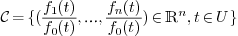
where  is the dimension of the ambient space
and
is the dimension of the ambient space
and  are univariate polynomials (with
coefficients in
are univariate polynomials (with
coefficients in  ).
).
If  , the rational curve is also called a
polynomial curve.
, the rational curve is also called a
polynomial curve.
Bézier curves are special types of rational curves, which use Bernstein bases to represent the polynomial functions.
A Bézier parametric curve is the image of a map  of the form
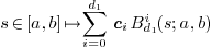
where  are the control points, and
  ,
,  are the Bernstein basis
elements of degree
are the Bernstein basis
elements of degree  for the interval
  .
.
A rational Bézier curve is constructed as follows:

where  are the weights of the control
points (usually
are the weights of the control
points (usually  ).
).
1.1.1.Axel format
<curve type="rational" color="0 255 0">
  <domain>0 1</domain>
  <polynomial>t</polynomial>
  <polynomial>t^2</polynomial>
  <polynomial>t^3</polynomial>
  <polynomial>1</polynomial>
</curve>
1.2.Rational surfaces
A rational curve is defined as the image of a map  of the form
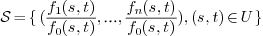
where is the dimension of the ambient space
and  are bivariate polynomials (with
coefficient in ).
are bivariate polynomials (with
coefficient in ).
1.2.1.Axel format
<surface type="rational" color="0 255 0">
 <domain>0 0 1 0 0 1</domain>
  <polynomial>s</polynomial>
  <polynomial>t</polynomial>
  <polynomial>s^2+t^2</polynomial>
  <polynomial>1</polynomial>
</surface>
1.3.Algebraic curves in the plane
An algebraic curve in  is defined by one
equation of the form:
is defined by one
equation of the form:

where  is a polynomial with coefficieints in
.
is a polynomial with coefficieints in
.
1.3.1.Example
Here is an image of the curve defined by the equation

1.3.2.Axel format
<curve type="algebraic" name="nice_curve_10">
  <domain>-4.1 4.2 -3.1 3</domain>
  <polynomial>-y^8+x^7-7*x^6*y+21*x^5*y^2-35*x^4*y^3+35*x^3*y^4
-21*x^2*y^5+7*x*y^6-y^7+8*y^6-7*x^5+35*x^4*y-70*x^3*y^2+70*x^2*y^3
-35*x*y^4+7*y^5-20*y^4+14*x^3-42*x^2*y+42*x*y^2-14*y^3+16*y^2
-7*x+7*y-2</polynomial>
</curve>
1.4.Algebraic curves in 3D
An algebraic curve in  is defined by two of
more equations of the form:
is defined by two of
more equations of the form:

The solution set of these equations is of dimension  .
In other words, the tangent linear space at almost all solution points
.
In other words, the tangent linear space at almost all solution points
 is a line.
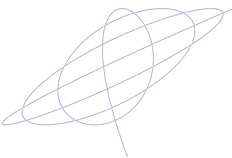
1.4.1.Example
Here we see two surfaces intersecting in a blue curve:
1.4.2.Axel format
<curve type="algebraic" color="0 0 255">
  <domain>-3 3.1 -3 3.1 -3 3.1</domain>
  <polynomial>10000*x^4+10000*y^4+10000*z^4-40000*x^2-40000*y^2*z^2-40000*y^2
-40000*z^2*x^2-40000*z^2-40000*x^2*y^2+207846*x*y*z+10000</polynomial>
  <polynomial>40000*x^3-80000*x-80000*x*z^2-80000*x*y^2+207846*y*z</polynomial>
</curve>
1.5.Algebraic surfaces
A general implicit surface is defined as the solution set of one equation:

where  is a subdomain of .
Usually
is a subdomain of .
Usually  is continous and enough differentiable
so
is continous and enough differentiable
so
An algebraic surface is a special case of an implicit surface where
 is a polynomial with coefficients in .
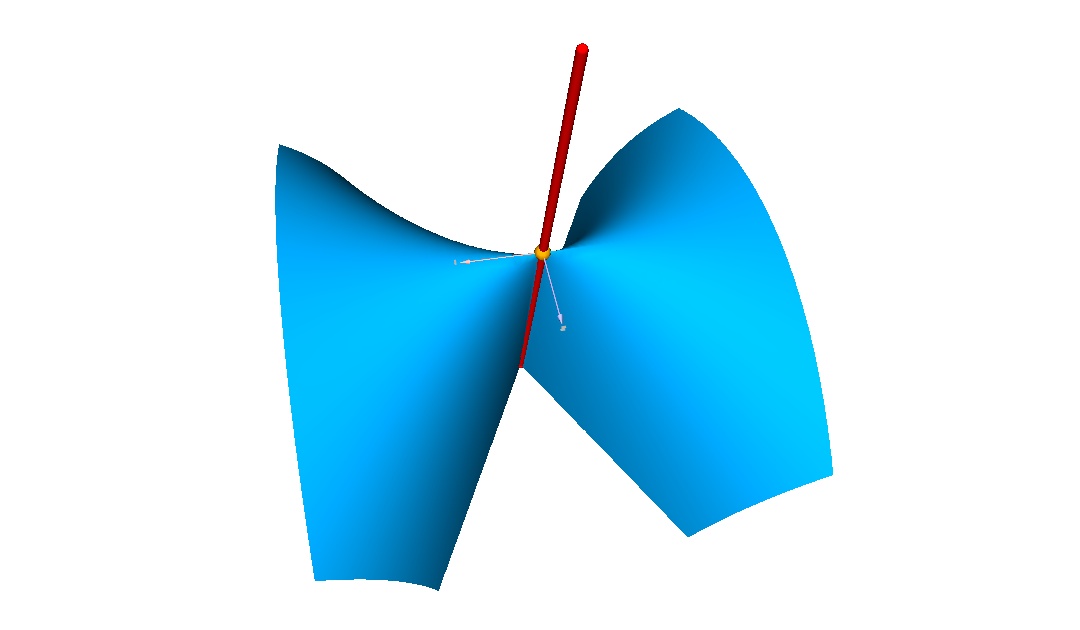
1.5.1.Example
Here is an example of a surface defined by the equation:

which is known as the Whitney umbrella.
1.5.2.Axel format
<surface type="algebraic" name="whitney umbrella" color="0 170 255" >
  <domain>-3 3 -3 3 -3 3</domain>
  <polynomial variables="x y z">x^2*y-z^2</polynomial>
</surface>
2.Algorithms
-
Topology and arrangement of algebraic curves
-
Topology of surfaces
-
Intersection of parametric surfaces
-
Auto-intersection of parametric surfaces